OpenFOAM As CFD Engine

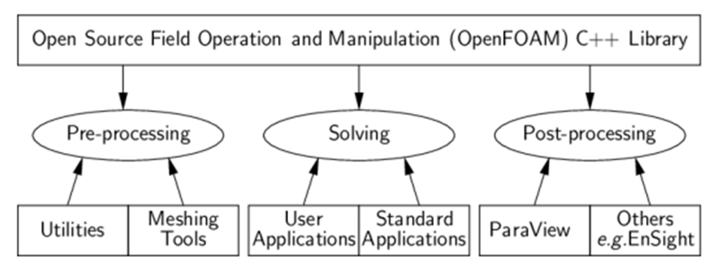
OpenFOAM (Open-Source Field Operation and Manipulation) is a powerful open-source computational fluid dynamics (CFD) software framework. It provides a comprehensive suite of numerical solvers and tools for simulating and analysing fluid flows, heat transfer, and other related phenomena. OpenFOAM is widely used in both academic and industrial settings due to its flexibility, extensibility, and the ability to customize and develop new solvers and models.

OpenFOAM is released under the GNU General Public License (GPL), making it freely available for use, modification, and distribution. This open-source nature encourages collaboration and innovation within the CFD community. It is designed with a modular architecture that allows users to add or modify components to suit their specific needs. New solvers, boundary conditions, turbulence models, and other features can be developed and integrated seamlessly into the framework. OpenFOAM offers meshing capabilities allowing users to generate complex structured and unstructured meshes for their simulations. Nevertheless, includes a variety of turbulence models, ranging from standard k-epsilon and k-omega models to more advanced Large Eddy Simulation (LES) and Direct Numerical Simulation (DNS) methods and provides a wide range of built-in solvers for various fluid flow and heat transfer problems. These include solvers for laminar and turbulent flows, compressible and incompressible flows, multiphase flows, and more.

Input parameters and boundary conditions

The foundational equations governing fluid flow are discretized and numerically solved within a three-dimensional spatial region encompassing the architectural structure, denoted as the computational domain. This domain is defined by six bounding surfaces, typically forming a cuboid shape. These bounding surfaces, except for the base of the domain, lack direct physical correspondence, leading to deviations from real-world conditions. These deviations introduce errors into the simulation of fluid flow, termed "domain errors." To mitigate these errors, it is imperative to position these non-physical bounding surfaces sufficiently distant from the architectural structure, thus minimizing their influence on the flow behaviour. However, excessive distancing of these boundaries could escalate the computational burden of the model. Therefore, the extent of the computational domain must be judiciously determined, considering both computational efficiency and the precision of the solutions.

The principles of computational wind engineering, as stipulated by well-established guidelines, emphasize the critical role of appropriately sizing the computational domain to ensure solution accuracy. These guidelines establish a connection between errors stemming from domain configuration and analogous issues observed in wind tunnel experiments, such as blockage effects within domains possessing constrained cross-sectional areas, and the artificial enhancement of local flow phenomena when inadequate space exists between the domain boundaries and the architectural model. Consequently, the determination of the minimum separation between domain boundaries and the architectural model, alongside the establishment of maximum blockage ratios, or a synergistic combination of both factors, serves to define the requisite domain size.

Mesh generation processes

The process of mesh generation typically involves two fundamental stages: the discretization of the computational domain and the incorporation of the studied structure within this domain.

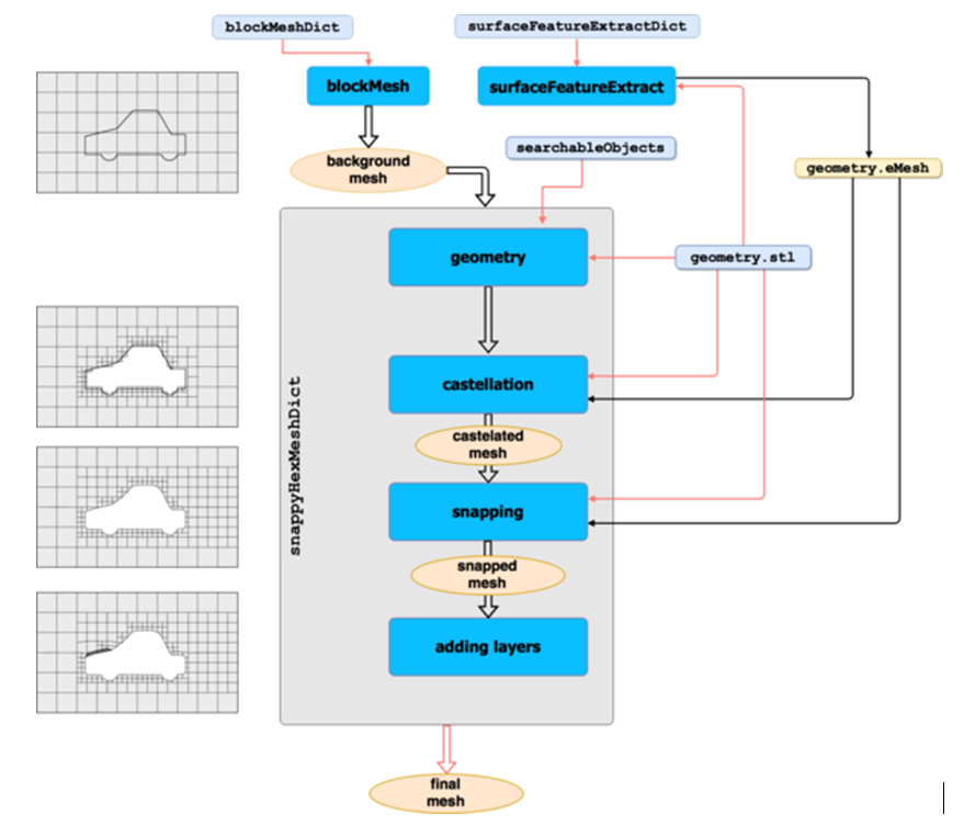
For this OpenFOAM employs two key tools: “blockMesh” and “snappyHexMesh”. These tools play a pivotal role in creating structured and unstructured grids, respectively, facilitating accurate simulations of complex fluid dynamics phenomena.

blockMesh is primarily utilized for generating structured grids. It employs a structured Cartesian coordinate system, allowing the creation of orthogonal hexahedral cells, which simplifies the numerical solution of partial differential equations. This tool works by partitioning the computational domain into a collection of blocks, and then further subdividing these blocks into cells through specification of vertices and edges. The block topology, along with boundary conditions and cell refinements, is defined in a dictionary file prior to executing the blockMesh utility. This approach is particularly well-suited for simpler geometries, where the Cartesian grid structure provides a clear representation of the domain.

On the other hand, snappyHexMesh is employed when more complex geometries are encountered, requiring unstructured grids for improved accuracy and flexibility. This tool is based on the concept of 'snap', which involves deforming an initial background grid to fit the geometry of interest.

Therefore, the meshing process involves the following stages:

• Background Mesh Generation: An initial grid is generated, which acts as a background mesh and covers the entire computational domain.

• Geometry Preparation: The target geometry is prepared in a specific format, which includes a surface description and relevant refinement parameters.

• Mesh Snapping: The initial background mesh is deformed, or 'snapped', onto the geometry's surfaces using iterative algorithms. This ensures that the mesh conforms accurately to the complex shape.

• Cell Layer Addition: After the surface snapping, a layer of prismatic or hexahedral cells can be added near the geometry's surface to capture boundary layer effects.

• Mesh Refinement: Localized mesh refinements can be applied to regions of interest, ensuring higher mesh resolution where necessary.

The overview of the meshing procedure via OpenFOAM

Turbulence modelling

Turbulence modelling is an essential component of Computational Fluid Dynamics (CFD) simulations used to predict the behaviour of fluid flows in various engineering applications. Turbulence refers to the chaotic change of field values in space and time at high velocities, a challenging phenomenon to accurately model and predict using traditional methods. CFD simulations aim to capture the complex interactions and fluctuations that arise in turbulent flows by employing various turbulence models.

In real-world scenarios, turbulence is ubiquitous and significantly impacts fluid behaviour, heat transfer, and mass transport.

Accurate prediction of turbulence effects is crucial for designing efficient and safe engineering systems, such as aircraft, vehicles, buildings, and industrial processes. However, simulating turbulence directly requires solving the Navier-Stokes equations for every individual turbulent eddy, which is computationally prohibitive for most practical applications. Turbulence models offer a compromise between accuracy and computational cost.

Overview of turbulence modelling approaches

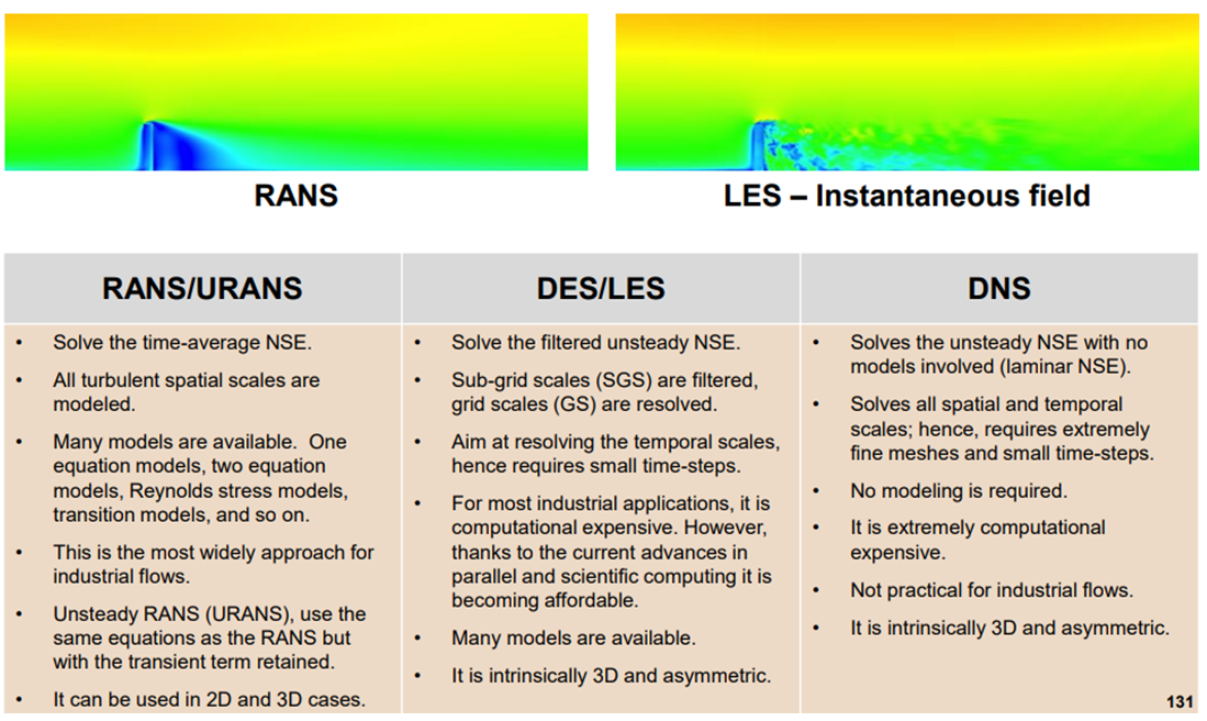
Turbulence models can be categorized into two main types: Reynolds-Averaged Navier-Stokes (RANS) models and Large Eddy Simulation (LES) models. RANS models average the flow variables over time and space to obtain the mean flow properties. These models solve for the mean flow field while providing additional equations to predict the turbulent fluctuations. While LES models simulate larger eddies explicitly while modelling smaller eddies. This approach is computationally more demanding than RANS models but can provide higher accuracy for complex flows. LES is suitable for capturing large-scale turbulence structures.

Selecting an appropriate turbulence model depends on factors such as the type of flow, geometric complexity, computational resources, and desired accuracy. Simple flows with well-defined geometries might benefit from RANS models due to their efficiency, while complex, unsteady flows might require LES for accurate predictions.

Turbulence modelling is not without challenges. Models often rely on empirical constants that might not be universally applicable. Some flows, particularly those involving separation, shock waves, or unsteady phenomena, can challenge turbulence models' accuracy. The choice of mesh resolution and boundary conditions also plays a critical role in obtaining meaningful results.

In summary, turbulence modelling is a vital aspect of CFD simulations, bridging the gap between computational feasibility and accurate prediction of turbulent fluid flows. Choosing the right model and understanding its limitations are crucial for obtaining reliable insights into complex fluid behaviour.

On of the most widely used turbulence models is the k-epsilon RANS model. It aims to predict the turbulent properties of a flow, primarily the turbulent kinetic energy (k) and the turbulent dissipation rate (ε). These two quantities are essential for characterizing the turbulence in the flow field. Here's a brief explanation of the k-epsilon model:

Turbulent kinetic energy (k): Turbulent flows consist of eddies and swirls of varying sizes. The turbulent kinetic energy represents the energy associated with these turbulent eddies.

Turbulent dissipation rate (epsilon): This represents the rate at which turbulent kinetic energy is converted into heat due to viscous dissipation. It is computed based on the gradients of velocity fluctuations in the flow field.

The k-epsilon model solves transport equations for k and epsilon, considering the effects of turbulence production, dissipation, and turbulent diffusion. The model involves the assumption of local equilibrium, which means that the turbulent production and dissipation are in equilibrium at each point in the flow field.

The k-epsilon model is relatively simple and computationally efficient, making it a popular choice for a wide range of engineering simulations. However, it may not accurately capture the complexities of certain turbulent flows, especially those with strong swirling or anisotropic behaviour. In such cases, more advanced turbulence models like the Reynolds Stress Model (RSM) or Large Eddy Simulation (LES) may be more appropriate. The choice of turbulence model depends on the specific flow characteristics and the level of accuracy required for the simulation.

Solvers

Computational Fluid Dynamics (CFD) solvers are pivotal components of numerical simulations that enable the study and analysis of fluid flow and its interactions with solid structures. These solvers encompass a diverse range of mathematical and computational techniques, offering the capability to simulate complex fluid dynamics scenarios that may be challenging or impractical to study through physical experiments alone.

CFD solvers work by discretizing the governing equations of fluid motion (Navier-Stokes equations) into a numerical grid or mesh that spans the computational domain. This mesh is composed of discrete cells or elements where fluid properties are computed and updated at discrete time steps. The choice of solver depends on the type of flow being simulated, the level of accuracy required, and computational resources available.