Analysis types

Elastic analysis

First order

The first order analysis calculates the structural response considering the initial stiffness of the model. It is advisable to run a first order analysis in order to check the model performance before executing more costly calculations (for instance eigenvalue analysis). The steps of the first order analysis are the following:

1. Calculation of first order (initial) stiffness matrices ($K_s^{el}$) of the finite elements in their local coordinate system
2. Compiling the global stiffness matrix ($K_s$) and nodal force vector ($P$) of the whole model by transforming the element stiffness matrices into the global coordinate system
3. Modifying the global stiffness matrix and nodal force vector considering the special boundary conditions (supports, continuity releases between the elements, prescribed displacements, temperature loads etc.)
4. Solution of the basic linear system of equations which writes the relationship between the applied nodal forces – known variables generated from the loads – and the nodal displacements – unknown variables ($U$) – in the global coordinate system for the global model (see section 8.2 Finite elements for the interpretation of nodal displacements and forces):

$K_sU=P \rightarrow U=K_{s}^{-1}P$

(1)

5. Calculation of the internal forces (and stresses) of the elements ($f^{el}$) in their local coordinate system by transforming the global nodal displacements of the element into local system ($u^{el}$) using their local stiffness matrices:

$f^{el}=K_s^{el}u^{el}$

(2)

Second order

The second order calculations take into account that the loaded and deformed structure can behave differently than the initial configuration. This effect can be considered as if the initial stiffness was changing during the loading history. The steps of the second order analysis are the following:

1. Performing the whole first order analysis as described in the previous section
2. Calculation of geometric stiffness matrices ($K_g^{el}$) of the finite elements in their local coordinate system by the internal forces of the elements ($f^{el}$)
3. Compiling the second-order global stiffness matrix ($K_s+K_g$) and nodal force vector ($P$) of the whole model by transforming the element stiffness matrices into the global coordinate system
4. Modifying the second-order global stiffness matrix and nodal force vector considering the special boundary conditions (supports, continuity releases between the elements, prescribed displacements, temperature loads etc.)
5. Solution of the basic linear system of equations which writes the relationship between the applied nodal forces – known variables generated from the loads – and the nodal displacements – unknown variables ($U$) – in the global coordinate system for the loaded and deformed global model (see section 8.2 Finite elements for the interpretation of nodal displacements and forces):

$(K_s+K_g)U=P \rightarrow U=(K_s+K_g)^{-1}P$

(3)

6. Calculation of the internal forces (and stresses) of the elements ($f^{el}$) in their local coordinate system by transforming the global nodal displacements of the element into the local system ($u^{el}$) using their local stiffness matrices:
   $f^{el}=K_s^{el}u^{el}$
7. If the difference between the new nodal displacements and the ones obtained earlier exceeds a certain limit repeat the calculations from step 2

Static eigenvalue – buckling analysis

In a mechanical interpretation the eigenvalue analysis approximates the elastic critical load levels where the structure is subjected to some modes of loss of stability. Mathematically it means that the second order equation of (3) has no unique solution because the second order stiffness matrix is singular. In Consteel linear eigenvalue analysis is performed considering one parameter, conservative loading and that the geometric stiffness matrix depends linearly on the load factor (λ):

$K_g(\lambda f)=\lambda K_g(f)$

(4)

In this case the eigenvalue analysis can be written in the following form:

$(K_s+\lambda K_g)U=0$

(5)

The solutions are certain critical load factors (buckling loads factor $\lambda_{cr}^i$) which make the second-order stiffness matrix singular and corresponding displacements (buckling shapes $U^i$).

The possible buckling shapes which can be calculated by this eigenvalue analysis are basically influenced by the considered second-order effects which are determined by the applied finite element. In the case of beam-column structures, the 7 DOF finite elements have the capability to consider all modes of global buckling shapes: flexural buckling, torsional buckling, lateral-torsional buckling, and any interactions of these.

Buckling sensitivity

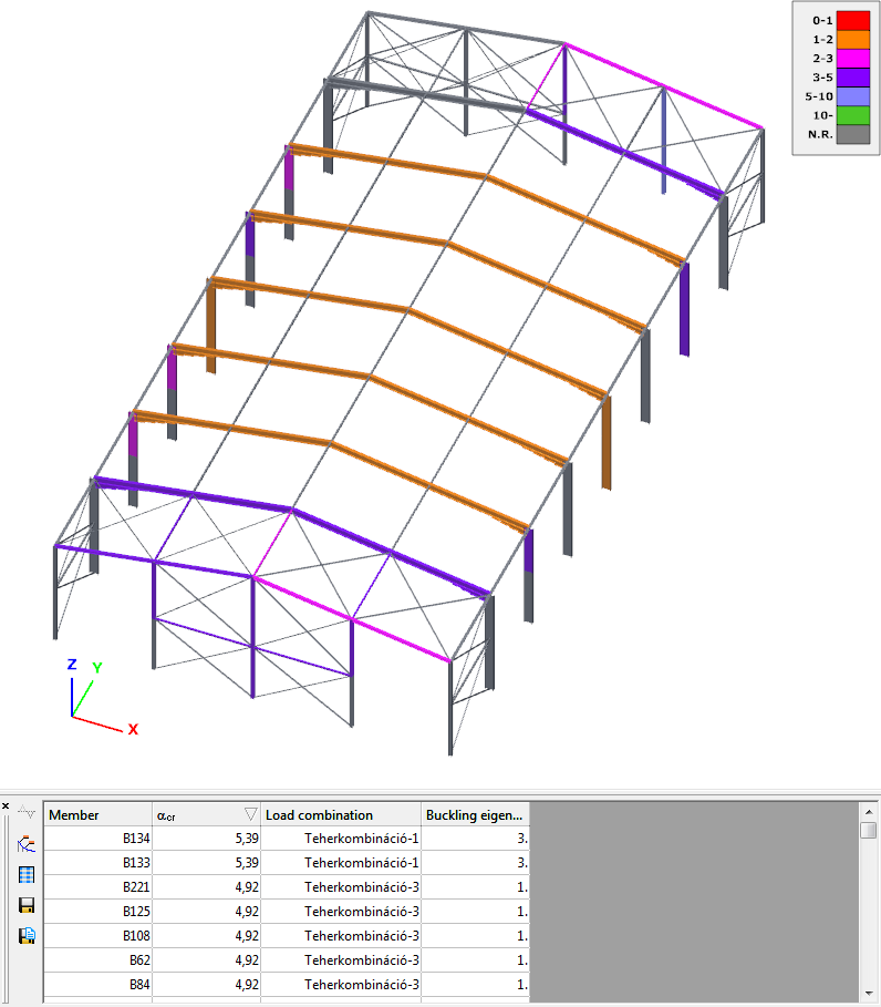
With the help of this function we get a summarized view of the buckling shapes of the structure, and for each member it gives which buckling shape of which combination is the most relevant for the stability analysis. Based on this, the program can automatically select the appropriate critical load factor for each member. See Global checks.

Imperfection sensitivity

This analysis determines the critical member and critical section for each of the eigenshapes. With the help of this analysis, the appropriate amplitude of the buckling shape-based imperfection can be calculated. The graph shows the stress-based utilization from the internal forces obtained by applying the eigenshape as an imperfection displacement load, where the cross-section corresponding to the highest utilization is given the value 100%.

Dynamic eigenvalue – vibration analysis

In a mechanical interpretation, the dynamic eigenvalue analysis approximates the eigenfrequencies where the structure is subjected to some modes of free vibration. In Consteel, linear eigenvalue analysis is performed considering the second-order stiffness matrix and the consistent mass matrix (M)

$((K_s+K_g)+\omega^{2}M)U=0$

(6)

The solutions of the equation are the eigenfrequencies ($\omega^i$) and the corresponding displacements (free vibration shapes $U^i$).

The possible vibration shapes obtained from this analysis are fundamentally influenced by the stiffness and mass matrix considered, which in turn is determined by the type of finite element used. For example, in the case of a 7DOF column-beam finite element, all global vibrational shapes can be considered: buckling, torsional buckling, twist, and their interaction.

Plastic analysis

To start a plastic analysis go to the Analysis Settings window of the Analysis tab. This requires the selection of the Plastic option of the Calculation Type drop-down menu.

Basics

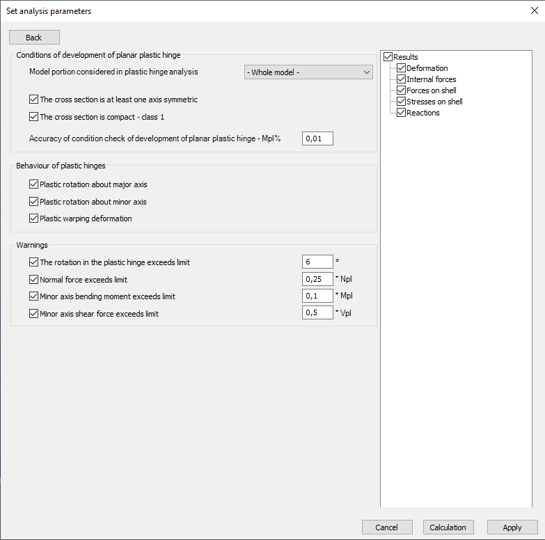
When plastic analysis is selected a plastic hinge analysis is performed considering planar hinges which may develop about the local y axis of the cross sections due solely to the major axis bending moment (My) – no other effects (like shear, normal force or minor axis bending) influence the formation of the hinge. The basic settings for the plastic analysis are available by pressing the three dots () button next to the Type of calculation combo on the Set analysis parameters dialogue.

In the first group, the conditions for the development of the plastic hinges can be set. The analysis can be set to look for plastic hinges in the whole model or only in a selected model portion (sub-model). Two options are available for the cross-section where hinges may develop: limited to at least singly symmetric (about the local ‘z’ axis) and to compact (AISC) or class 1 (EC) sections. According to the usual standard specifications, these last two conditions must be met in order to perform a plastic hinge analysis. The accuracy of the calculation can also be set as a percentage of the plastic bending resistance (Mpl).

In the second group, the mechanical behavior of the plastic hinges after formation can be set. Since the planar hinges are part of a spatial model (the term “planar” refers only to the formation of the hinges), their spatial mechanical behavior after formation should be defined (spatial hinges). Accordingly, the formed hinges can rotate around the major axis (in the original plane of source bending moment My), or around the minor axis together with free warping deformation. With the help of the latter two options, it can be realistically taken into account that a full-yielded flange in an I-shaped section practically allows the minor axis rotation and warping behavior. These options influence the out-of-plane behavior of the model only (for example, in the case where the buckling of a structural member develops next to a plastic hinge perpendicular to the plane of the hinge).

The third group of options offers warning displays. These warnings are displayed if the development of plastic hinges is significantly affected by effects other than the major axis bending moment (My) during the whole hinge history.

In the fourth group of options, the important results can be selected which have to be saved and displayed for all the stages. In the case of larger models and the possibility of a large number of hinges, the number of results can increase significantly so it is advisable to carefully choose the really important ones.

First order

Mathematically, it is done similarly as described for elastic calculation, but with the big difference that it not only analyzes the specified load but it also changes (increases or decreases) the specified load step by step until the structure becomes unstable due to the plastic hinges.

The solution process is as follows:

1: A first-order elastic analysis is performed according to the load combination specified by the user, and then the obtained bending moment values My about the strong axis are compared with the plastic moment resistance of the section of every finite element according to the criteria in the first group.

2a: If the stresses calculated at the load level specified by the user do not meet the conditions for the formation of the plastic hinge(s) at any point of the elements selected for plastic analysis, Consteel raises the load level in steps until the first plastic hinge is formed.

2b: If there is a point at the user-specified load level where the plastic hinge would form, Consteel reduces the load level in steps until the load level is found when the first plastic hinge is formed.

3: At the found load level $(\alpha *M_{yEd})$ Consteel places hinges on all current finite element points where the conditions for the formation of the plastic hinges are given according to the parameters of “Behavior of plastic hinges”, which is used in the analysis for additional load steps. Due to the placement of the hinges, the global stiffness matrix of the structure is updated and another level of calculation is started. The placed joints are shown on the structure and the next calculation step starts.

4: Consteel further increases the load through the -α- load factor using the changed stiffness matrix until the load level for the formation of the next plastic hinge is reached.

5: As in point 3, place joints on the newly found nodes, update the stiffness matrix, and continue the iteration according to point 4.

The plastic analysis ends when the resulting structure including the plastic hinges becomes unstable as a result. If the value of the final load factor thus obtained is less than 1.00, the structure is unstable, and the first-order calculation ends without result. A message alerts the user.

During the iteration, when the program reaches the load factor value of 1.00, the current internal force values are saved because the global design must be performed at this level, i.e. at the specified load level. These internal forces will be the basis for the buckling analysis to be performed in the next step.

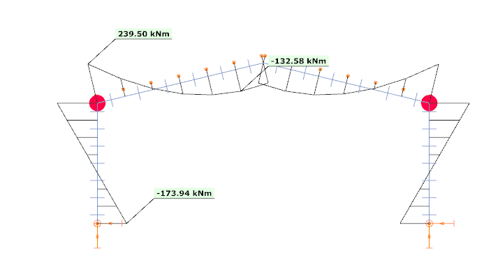
You can view the history of each load level step, its associated load factors, and the plastic hinges formed during the steps by selecting the “Plastic hinges” option from the Analysis Types drop-down menu.

Second order

Coming soon!

Static eigenvalue – buckling analysis

The iteration described for the first-order analysis is performed up to a load factor of 1.00, which corresponds to the specified load level. Using the first-order Ks corresponding to the static model valid at this load level and the Kg matrices calculated for the corresponding internal force distribution, the calculation is performed as described in the elastic analysis.